• The Code
  • Setup
• JAX Basics
• How to Write Bad JAX
  • Basic JAX and MJX
  • Using JIT to Speed Things Up
• How to Write Better JAX
  • Parallelism
  • Jitting the Whole Thing
  • Looping with Scan
• A Full Data Collection Loop
• Conclusion

Most roboticists know MuJoCo, Google’s simulation library for rigid-body robotics. Fewer have spent much time with JAX, Google’s numerical computing library for scientific computing and machine learning. JAX is fiddly, but for parallel simulation it can be outrageously fast.

I’m currently working on a basic world model, which means I need to collect a bunch of simulation data to train it. In this post I’ll show how JAX, via its MuJoCo backend MJX, gives us a neat way to do that data collection quickly. Here’s a companion Google Colab you can run to try things for yourself.

The timings below are steady-state after jit compilation. I’m reporting amortised time per environment step: total rollout wall-clock time divided by n_steps * n_envs (and by n_runs in the final example). For the single-environment examples, n_envs = 1.

The Code

Setup

import jax
from mujoco_playground import registry

env_cfg = registry.get_default_config("CartpoleBalance")
env = registry.load("CartpoleBalance", config=env_cfg)

In this code I’m using mujoco_playground for a convenient MuJoCo/MJX environment. We load Cartpole — a basic environment offered in many RL codebases. The env object will be familiar to RL practitioners: It exposes a step method which takes an action and increments the simulation. Cartpole itself looks like this:

JAX Basics

As mentioned above, JAX largely resembles NumPy, which might make you wonder why you should care about it. What makes JAX special is its transforms. Transforms let you modify NumPy-style code to use a GPU for a big speedup. The three most important transforms for our purposes are:

• jit: a ‘just-in-time’ compiler traces through your Python code and compiles it down to a faster representation which can run on GPU. Jit will make the first run of a function pretty slow while the compiler writes its new code, but subsequent calls are much faster.
• vmap: short for ‘vectorising map’, it makes your code run in parallel so you can reap the benefits of using a GPU.
• scan: ‘JAX-ifies’ Python ‘for’ loops, netting a speedup for sequential jobs like simulation.

How to Write Bad JAX

In the intro I mentioned that JAX is fiddly. It’s worth it, but it is absolutely fiddly. To illustrate that point, I’ll first write a naive implementation that looks like good old NumPy. Then we’ll JAX-ify our code step-by-step and watch the performance tick up.

Basic JAX and MJX

First let’s see what it looks like to run an episode in our environment. For these examples we only care about broad data collection, so I’ll just use random actions.

n_steps = 10
# JAX relies on manual RNG management. This is annoying, but it means
# everything is deterministic.
key = jax.random.key(0)
reset_key, key = jax.random.split(key)

# We reset the environment at the start to get it in a fresh state
state = env.reset(reset_key)

for t in range(n_steps):
    # Select a random Gaussian action
    action_key, key = jax.random.split(key)
    action = jax.random.normal(action_key)

    # Step the environment
    state = env.step(state, action)

Time per step: 1.4s. This is pretty simple, and hopefully fairly intuitive! It shows off one JAX quirk — manual RNG management via keys. Reusing a key gives you repeat randomness, so you need to do a painful dance of splitting keys every time you do something random. It’s irritating, but the determinism you get from this pays for itself in the long run. And it enables cool tricks like communicating massive amounts of data purely via single integer keys. There’s a catch, however: This is slow as sin. On my MacBook Pro, it takes 14.1 seconds for 10 steps. Let’s track that stat — seconds per step — to see how things improve.

Using JIT to Speed Things Up

As nice as our code is, we’re not making use of our wonderful JAX transforms; that’s why it’s so slow. For the first improvement, let’s jit:

n_steps = 1_000 # We can now run for more steps without dying of old age

# The only real change - wrap our env functions in jax.jit
reset = jax.jit(env.reset)
step = jax.jit(env.step)

key = jax.random.key(0)
reset_key, key = jax.random.split(key)

state = reset(reset_key)

for t in range(n_steps):
    action_key, key = jax.random.split(key)
    action = jax.random.normal(action_key)

    state = step(state, action)

Time per step: 0.3ms. Just by wrapping the step and reset functions in a jax.jit call, our code is about 5000x faster. Not bad. However, if you run this code by itself in a notebook, you might not see the same benefit at first. Because jit has to trace the code and compile it before running it, the first run is much slower, about 2s on my machine. After that, our loop gets much faster.

If you’re used to MuJoCo, you might have a more pressing thought: ‘This is still slow.’ This single-environment loop is 40x faster in vanilla MuJoCo. To get value from MJX, we need to get JAX-ier.

How to Write Better JAX

Parallelism

The big advantage of JAX is that it can natively parallelise our code. But so far we’re running everything one step at a time. How 2000s. Instead, let’s use our next transform, vmap, to actually benefit from GPU parallelism. This one is still pretty simple — MJX is built from the ground up to work with vmap:

# Define how many environments we want to run in parallel
n_envs = 256
reset = jax.jit(jax.vmap(env.reset))
step = jax.jit(jax.vmap(env.step))

key = jax.random.key(0)
reset_key, key = jax.random.split(key)

# Now, for the vmapped function we're giving it `n_envs` keys, instead of just 1.
state = reset(jax.random.split(reset_key, n_envs))

for t in range(n_steps):
    # Similarly, here we output an action with a first dimension
    # of n_envs. That corresponds to one action
    # for each environment we're running.
    action_key, key = jax.random.split(key)
    action = jax.random.normal(action_key, shape=(n_envs, 1))

    state = step(state, action)

Time per step: 1.25μs. About 240x faster than our last version. Just by telling JAX we want parallelism, we can run loads of simulations alongside each other and reap the benefits of parallelism. You’re only really limited by your hardware. On my MacBook I get gains up to 256 environments, but on an L4 GPU I can run 8,192 simulations at once.

Jitting the Whole Thing

Now we’re starting to cook. But to get even faster, there’s more to do. First, we’ve jitted our environment functions step and reset, but the rest of our code is still normal Python. We can do better. The JAX-y thing to do now is to wrap all our code in one function, which we can then jit all together.

# Define how many environments we want to run in parallel
n_envs = 256

# only doing short rollouts to limit jit's unrolling
n_steps=10 

@jax.jit
def run_episode():
    reset = jax.vmap(env.reset) # because we jit the outer function, we don't need to
    step = jax.vmap(env.step)   #  jit the environment functions separately any more.

    key = jax.random.key(0)
    reset_key, key = jax.random.split(key)

    state = reset(jax.random.split(reset_key, n_envs))

    for t in range(n_steps):
        action_key, key = jax.random.split(key)
        action = jax.random.normal(action_key, shape=(n_envs, 1))
        state = step(state, action)

    return state

run_episode()

Time per step: 1.1μs. Jitting our whole function hasn’t given us an incredible speedup, but it sets us up for the next round of improvements. The keen-eyed reader will notice that we’ve capped the number of forward steps to 10, rather than the 1,000 we were using before. That’s because, behind the scenes, jax.jit unrolls Python ‘for’ loops:

# A function like this...
@jax.jit
def fn():
    for i in range(5):
        do_something(i)

# ...looks like this internally after unrolling.
def jitted_fn():
    do_something(0)
    do_something(1)
    do_something(2)
    do_something(3)
    do_something(4)

That’s OK for a short rollout, but if you do it for 1,000 steps the compiled code becomes enormous, and JAX will gladly eat all your RAM for lunch. Give it a test if you’re coding along at home (and enjoy tormenting your computer).

Looping with Scan

For a fully JAX-native implementation we need to use our final, most complex, transform: scan. scan is JAX’s version of a ‘for’ loop. It’s powerful but awkward: it requires very specific function definitions and inputs. It leans on the idea of a carry (which is passed from one iteration to the next), x (any extra inputs — this defines the length of the loop) and y (some data you want back out of the scan). JAX will automatically stack the y from each timestep into an output array.

def f(carry, x): ...
carry, ys = jax.lax.scan(f, init, xs)

# Internally, scan here looks like this.
def scan(f, init, xs):
  carry = init
  ys = []
  for x in xs:
    carry, y = f(carry, x)
    ys.append(y)
  return carry, np.stack(ys)

scan is a bit awkward, so you really just need to write it yourself to get used to the syntax. I recommend writing out a basic ‘for’ loop and mapping it onto the Python version in the docs. Once you’ve figured out what goes where (What’s the carry? Do I need an x? What’s y?) you’re ready to convert it into a scan. Here’s our simulation loop written with scan:

n_envs = 256
n_steps = 1_000

@jax.jit
def run_scan_episode():
    reset = jax.jit(jax.vmap(env.reset))
    step = jax.jit(jax.vmap(env.step))

    key = jax.random.key(0)
    reset_key, key = jax.random.split(key)

    # Set up our 256 environments
    state = reset(jax.random.split(reset_key, n_envs))

    # First we need to define a function to scan. Scan runs
    # along sequences - in our case the sequence is time, so we'll define
    # a one-step function.
    def simulate_step(state, action_key: jax.Array):
        "Simulates an individual time step"
        actions = jax.random.normal(action_key, shape=(n_envs, 1))
        next_state = step(state, actions)

        # Scan functions return two parts - a carry which is reused
        # at the next step, and data to be concatenated together.
        return next_state, {
            "obs": state.obs,
            "action": actions,
            "next_obs": next_state.obs,
        }

    # We set up a random key for each time step. This is what we'll 'scan'
    # along - the first dimension of our keys array
    keys = jax.random.split(key, n_steps) # shape (1000,)
    state, data = jax.lax.scan(simulate_step, state, keys)
    return data

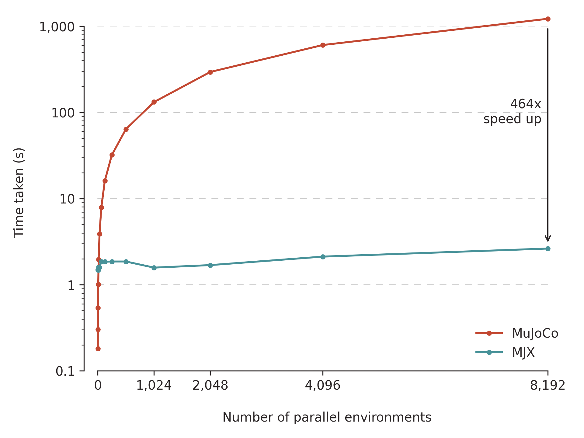
Time per step: 700ns. Here, our carry is the state (the thing being updated every step), x is the key used to sample an action, and y is our output data (recording $(s, a) \rightarrow s^\prime$ tuples). That’s exactly the dataset shape a one-step world model needs: current observation, action, next observation. JAX is comfortable with dictionaries of Arrays (or ‘PyTrees’ in JAX-speak), so we can output a dict from our step function and scan will magically stack the arrays for each timestep. With that, we’re basically done, with another 50% speedup! In the end, we’re ~2,000,000x faster than the naive loop, and 460x faster than normal MuJoCo. Like all benchmarking tasks, the right way to show how far we’ve come is one of those bouncy-ball visualisations:

A Full Data Collection Loop

For extra credit we might like to collect even more data, but our previous examples are limited by how many environments we can run in parallel. To get our complete data collection loop, we’ll add one more scan to repeat the loop. This final snippet is a bit more complex, but it only uses the ideas we’ve covered so far:

import einops

n_runs = 10
n_envs = 8192
n_steps = 1000

@jax.jit
def collect_random_scan_data():
    reset = jax.vmap(env.reset)
    step = jax.vmap(env.step)

    def simulate_step(state, action_key: jax.Array):
        "Simulates an individual time step"
        actions = jax.random.normal(action_key, shape=(n_envs, 1))
        next_state = step(state, actions)
        return next_state, {
            "obs": state.obs,
            "action": actions,
            "next_obs": next_state.obs,
        }

    def simulate_trajectory(key, _):
        "Simulates an entire trajectory"
        key, reset_key, rollout_key = jax.random.split(key, 3)

        state = reset(jax.random.split(reset_key, n_envs))
        keys = jax.random.split(rollout_key, n_steps)

        # Scan 1 outputs arrays of shape (n_steps, n_envs, ...)
        _, ep_buffers = jax.lax.scan(simulate_step, state, keys)
        return key, ep_buffers

    # Scan over multiple trajectories instead of using vmap so
    # we can collect many episodes without blowing our VRAM budget.
    key = jax.random.key(0)

    # Scan 2 runs more of Scan 1 in a loop, giving us arrays
    # of shape (n_runs, n_steps, n_envs, ...)
    _, buffers = jax.lax.scan(simulate_trajectory, key, length=n_runs)

    # The buffer contains arrays of shape: (n_runs, time, n_envs, ...)
    # Let's stack them so we get:          (batch, time, ...)
    buffers = jax.tree.map(
        lambda a: einops.rearrange(a, "r t e ... -> (r e) t ..."), buffers
    )

    return buffers

Time per step (MacBook): 720ns. Time per step (Colab L4 GPU): 32ns.

Conclusion

Mission Accomplished. This is a great foundation for training a world model — we’ve now got a fast, efficient means of collecting loads of simulation data in parallel. The tricks used here — jit, vmap and scan — will show up again as we build out JAX models. And if we want to collect on-policy data, we just need to swap in an action = policy(state) and we’re off to the races.

Mission Un-complished. Just reading a blog post, JAX looks pretty good. But it has a steep learning curve and sharp edges. Additionally, MJX has some issues of its own: it typically runs at lower floating-point precision, and is missing features from normal MuJoCo. That said, the ability to run so many sims in parallel is enormously powerful, especially for data-hungry RL agents.

Thanks for reading! Hopefully you’ve found this tour around JAX and MJX useful.