• What Is a World Model?
• Learning to Model the World
  • Network Definition
  • The Training Loop
• Using MPC to Derive a Policy
  • World Model: Rollout!
  • Generating Actions
  • Deriving Our Policy
• How Does It Do?
  • The Bigger Picture

What Is a World Model?

There are lots of competing definitions of world models, and frankly the term is becoming so diluted it’s increasingly useless. Fei-Fei Li’s world models focus on 3D visual reconstruction. Yann LeCun’s JEPAs learn and predict underlying latent representations from video. Genie 3 is more action-oriented (check out my write up here). Credible people like Kevin Murphy reckon LLMs constitute world models. For their part, Goldman Sachs think that… wait what? What bubble!?

Anyway, for my world model I’m going to take a more traditional Reinforcement Learning view - that means we’re talking about a state $s$, and an agent taking an action $a$. In that universe, a world model is fundamentally defined by predicting what the next state will be following a state-action pair:

In this blog, we’ll train a simple model $f_\theta$ and use MPC to transmute it into a policy. We can do something cool here; by training a world model only on random data, we’ll derive a working policy without our data collection ever being designed for any particular task. In some sense, that’s what we do as humans. We think about what we want to get done, use our world knowledge, and squish them together to come up with a novel solution. We do that without needing to know the problem in advance, unlike typical RL solutions where the reward function is usually a core part of training. As per usual, the code is available at this notebook if you’d like to run it yourself.

Learning to Model the World

Network Definition

I covered fast data collection using MJX in my last post, so I won’t dwell on the details here. Our data collection will be random, looking something like this.

We’ll store and access transitions $(s, a, s’)$. With data collected, we can train a basic neural network to predict $s’$ given the initial state-action pair. I’m using Google’s flax.nnx library for this because it works well with the JAX transforms we’re using elsewhere.

# Define one layer of the network.
class LayerBlock(nnx.Module):
    "A single linear layer using batchnorm for stable training."
    def __init__(
        self,
        in_features: int,
        out_features: int,
        activation_fn: Callable,
        rngs: nnx.Rngs,
        bn: bool = True,
    ):
        self.layers = nnx.List(
            [
                nnx.Linear(in_features, out_features, rngs=rngs),
                nnx.BatchNorm(out_features, rngs=rngs) if bn else nnx.identity,
                activation_fn,
            ]
        )

    def __call__(
        self, x: Shaped[Array, "... InFeatures"]
    ) -> Shaped[Array, "... OutFeatures"]:
        for layer in self.layers:
            x = layer(x)
        return x

# Stick a few layers together for our full network.
class OneStepWorldModel(nnx.Module):
    def __init__(self, rngs: nnx.Rngs):
        self.layers = nnx.List(
            [
                LayerBlock(6, 32, activation_fn=nnx.swish, rngs=rngs, bn=True),
                LayerBlock(32, 64, activation_fn=nnx.swish, rngs=rngs, bn=True),
                LayerBlock(64, 32, activation_fn=nnx.swish, rngs=rngs, bn=True),
                # Skip batchnorm and an activation function for the output layer
                LayerBlock(32, 5, activation_fn=nnx.identity, rngs=rngs, bn=False),
            ]
        )

    def __call__(
        self,
        obs: Shaped[Array, "... StateDim"],
        action: Shaped[Array, "... ActionDim"],
    ) -> Shaped[Array, "... StateDim"]:
        # Stack the state and action into one array
        x = jnp.concatenate([obs, action], axis=-1)
        for layer in self.layers:
            x = layer(x)

        obs = x + obs  # predict the delta
        # normalise the sin and cos components (axes 1,2) to the unit circle
        sincos_norm = jnp.linalg.norm(obs[..., 1:3], axis=-1)
        obs = obs.at[..., 1].set(obs[..., 1] / sincos_norm)
        obs = obs.at[..., 2].set(obs[..., 2] / sincos_norm)
        return obs

The Training Loop

To train the model, I’m using a basic loss function, which just computes the squared distance between the model prediction $f_\theta(s_t, a_t)$ and the true next state $s_{t+1}$. We should really normalise each dimension of the state for this calculation (say the cart velocity was 10x larger than everything else — without normalisation it will dominate the prediction error, and the model will overly focus on it). But the un-normalised loss is good enough for this demo.

We’ll combine our loss function with a fairly bog-standard nnx training loop. The big difference vs. PyTorch is the use of nnx.value_and_grad — we tell JAX to give us the gradient over a specific function, rather than computing a loss and calling loss.backward(). For more on Torch vs JAX, check out this post.

model = OneStepWorldModel(nnx.Rngs(0))

n_train_steps = 2000
# Use a simple learning rate schedule, which halves halfway
lr_schedule = optax.piecewise_constant_schedule(3e-4, {1000: 0.5})
tx = optax.adamw(lr_schedule)
optimizer = nnx.Optimizer(model, tx, wrt=nnx.Param)

# value_and_grad returns the backprop gradients from our loss function
@nnx.value_and_grad
def loss_fn(model, batch):
    pred = model(batch["obs"], batch["action"])
    squared_distances = jnp.linalg.norm(batch["next_obs"] - pred, axis=-1)
    return squared_distances.mean()


@nnx.jit
def train_step(model, optimizer, key):
    batch = sample_batch(buffers, key)
    loss, grads = loss_fn(model, batch)
    # This is where the model weights actually get updated.
    optimizer.update(model, grads)

key = jax.random.key(0)
for _ in range(n_train_steps):
    step_key, key = jax.random.split(key)
    train_step(model, optimizer, step_key)

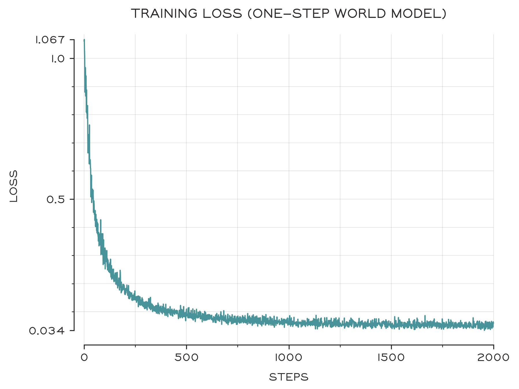
And we get a nice looking loss curve. It looks like our network has learned to model something, but loss is pretty meaningless — we care about results! To assess the usefulness of our world model, let’s use it to control a cart.

Using MPC to Derive a Policy

To get a policy out of our model, we’ll turn to model-predictive control, or MPC. I’ve written a more in-depth blogpost on MPC, but as a refresher, this is the procedure:

1. Generate possible sequences of actions.
2. Use our world model to figure out which states would arise if we took those actions.
3. Score each trajectory with a reward function.
4. Choose the action which leads to the best trajectory.
5. Repeat.

World Model: Rollout!

Our model estimates the next state given a state-action pair

Well, we can stick that back into our world model…

…and so on and so forth, unrolling our model to predict a trajectory of states. In code, that looks like this (using nnx.scan instead of a Python for loop).

@jax.jit
def rollout(
    model_graphdef: nnx.GraphDef,
    model_state: nnx.GraphState,
    initial_obs: Shaped[Array, "... StateDim"],
    actions: Shaped[Array, "... Time ActionDim"],
) -> Shaped[Array, "... Time StateDim"]:
    # This assert will freak out if one of our input arrays is the wrong shape
    chex.assert_equal_shape_prefix([initial_obs, actions], actions.ndim - 2)

    # Use of nnx.merge means we can use the functional API and rely on
    # normal JAX jit, which is slightly faster.
    model = nnx.merge(model_graphdef, model_state)

    # Usually faster to unroll along time on the first dimension, and
    # lax.scan requires it, so I've formed the habit.
    actions = rearrange(actions, "... T A -> T ... A")

    # Let's propagate batch stats across time steps
    state_axes = nnx.StateAxes({nnx.BatchStat: nnx.Carry, ...: None})

    # Use scan to unroll along the time dimension.
    @nnx.scan(in_axes=(state_axes, nnx.Carry, 0))
    def unroll(model, obs, action):
        next_state = model(obs, action)
        return next_state, next_state

    _, state_trajectory = unroll(model, initial_obs, actions)

    # Put the batch dimension on the first axis - no real need but
    # it just feels weird not to.
    return rearrange(state_trajectory, "T ... A -> ... T A")

Generating Actions

Note that, to give our model something to unroll over, we also need to give it some actions. Cartpole is simple, so we don’t need to get too fancy. We’ll generate random action sequences and use the world model to evaluate them. This technique is called random shooting, and it’s the simplest version of action sampling. Smarter alternatives like CEM or MPPI do more active optimisation on their action sequences which is relevant for higher dimensional spaces, but they’re overkill for our needs.

def gaussian_action_samples(
    key: jax.Array,
    horizon: int = 5,
    n_samples: int = 128,
    std: float = 0.2,
    mean: float = 0.0,
):
    shape = (n_samples, horizon, 1)  # 1 for action dim
    samples = mean + std * jax.random.normal(key, shape=shape)
    # cumulative sum over the horizon to accumulate a random walk
    samples = jnp.cumsum(samples, axis=-2)
    return jnp.clip(samples, -1, 1) # Cartpole actions are bounded between [-1, 1]

We’ll also want to define a reward function so our policy knows what’s good and what’s bad. For Cartpole, we’re usually trying to keep the pole vertical. We’ll call the angle of the pole $s_\phi$, giving us a simple reward function

def upright_reward_fn(
    obs: Shaped[Array, "... Time StateDim"],
) -> Shaped[Array, "... 1"]:
    pole_angle_cos = obs[..., 1]
    upright = (pole_angle_cos + 1) / 2
    return upright.mean(axis=-1)  # average over time steps

Deriving Our Policy

Now we have all the pieces for our policy. We just need to generate a random set of actions $a=(a_1, \dots, a_H)$, score the resultant states $(s_2, \dots, s_{H+1})$, and then pick the best action:

And then we simply select next action $a_1^*$. In code:

@jax.jit(static_argnames="reward_fn")
def simulate_policy(
    key,
    model_graphdef: nnx.GraphDef,
    model_state: nnx.State,
    reward_fn: Callable = upright_reward_fn,
):
    horizon = 5
    n_samples = 1024
    n_steps = 1000

    # Get initial state
    state = env.reset(key)

    def policy_step(state, key):
        initial_obs = state.obs
        initial_obs = repeat(initial_obs, "... S -> ... N S", N=n_samples)

        # sample a Gaussian trajectory
        actions = gaussian_action_samples(key, n_samples, horizon, std=0.5)

        state_trajectory = rollout(model_graphdef, model_state, initial_obs, actions)

        # score trajectory based on highest average reward
        rewards = reward_fn(state_trajectory)
        best_ix = rewards.argmax()
        best_actions = actions[best_ix]
        next_action = best_actions[0]
        state = env.step(state, next_action)
        return state, {"state": state, "action": next_action}

    keys = jax.random.split(key, n_steps)
    _, states = jax.lax.scan(policy_step, state, xs=keys)
    return states

How Does It Do?

OK so, we’ve put in all this effort — does it actually work?? Let’s review an instant replay:

I’d say that’s pretty good. We’ve asked our policy to keep the pole upright, and it does as requested, although it’s a bit wobbly off the rip. There are a number of simple improvements we could consider:

• Our data was driven by a random policy, so most of it is dissimilar to the states the policy encounters: a controlled, upright position. We can run more episodes with the model-derived policy and train a model with a blend of old and new data. That newer model will be more familiar with the kinds of state the policy ends up in, so it can make better predictions.
• We’re training our model on a simple one-step prediction error, but we actually want to unroll it over a whole horizon. Instead of training on single $(s, a, s’)$ transitions, we could train our model on longer prediction horizons — that’s what we ultimately care about.
• As mentioned above, the state we use in the loss function isn’t normalised. That’s an easy fix - just divide by the standard deviation of each of the state components in the dataset (jnp.std(buffers['state'], axis=-1)).
• Our action sampling strategy is pretty bad. Cartpole only has a 1-dimensional action space, so we can get good coverage of the space with a brute-force approach like random shooting. But on real problems our action space is far larger. There’s a more subtle issue too: with random shooting, our first action doesn’t really have anything to do with the rest of its sequence. Maybe the best trajectory happens to pick a rubbish first action, then loads of great ones afterwards — but then we only take the first action and discard the rest. Whoops. That’s where smarter approaches which actively optimise an action trajectory become a lot more attractive.

The Bigger Picture

Those are all sensible tweaks, but I think there’s a more interesting challenge. Let’s test our model with a harder task: can it transfer to a reward function which demands that the pole stays down?

Err. No. It can’t transfer at all.

What’s going wrong? Well, our policy is completely myopic. Our sim is operating at 100Hz, and we’re predicting over a 5 step horizon, so we’re only planning 0.05s ahead. That short horizon is OK for keeping upright: we start close to the optimal position, and the agent just needs to oppose movement in the bad direction. But for the downwards task, it’s too short-sighted. If our agent had a brain, it would be all fast-twitch nerves and no grey matter.

To address this failing, I think we need to get hierarchical. That means moving beyond one single model, to multiple models operating on different levels of temporal abstraction. That could be a small one running at 100Hz to do the fast motor control, as well as a big, slow model that thinks ahead. The big one tells the small one what to do, and together they should be able to handle tougher problems. That’s my theory at least, and it’s what I’m going to work on for the next post in this series. I’d also like to try MPC on some harder environments — Cartpole is fine, but I think we can do better.

Thanks for reading. I hope you found this useful, interesting, or at least not completely risible.